Vector spaces

A vector space, sometimes also called a linear space, is a set of elements that must satisfy certain properties, thanks to which the elements of the set, which we call vectors, behave “nicely”.

An example of a vector space

Before we define a vector space, let’s look at an example of one that you should already know from school, except that you may not know it is a vector space. They are the ordinary vectors in the plane.

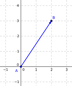
By a vector in the plane we mean an ordered pair (a, b), where a, b ∈ ℝ. These are any coordinates in the space ℝ² (meaning the Cartesian product ℝ × ℝ). We can represent such a vector by an arrow from the point (0, 0) to the point (a, b). The vector (2, 3) would look like this:

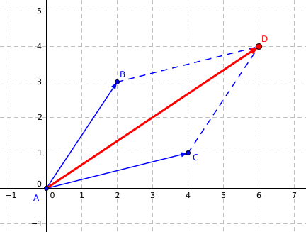
We know that vectors can be added using the rule (a, b) + (c, d) = (a + c, b + d). The sum of vectors (2, 3) + (4, 1) would be equal to the vector (2 + 4, 3 + 1) = (6, 4). Graphically we would show it like this:

We can also work out a scalar multiple of a vector, k times the vector, where k is a real number. We write k times a vector as k · (a, b). The result is a new vector, defined as k · (a, b) = (k · a, k · b). Graphically, the vector gets “stretched”, “shortened” or changes direction. If we have the vector u = (2, 3), then the vectors 2 · u, $\frac{1}{2}u$ and −1 · u look like this:

We will prove later that the set of all vectors ℝ² with the operations defined in this way forms a vector space. First we define a vector space, and then we will illustrate the individual properties on the vector space ℝ².

Definition of a vector space

A vector space (or linear space) is a non-empty set V whose elements we call vectors. There must also be two operations on the set: addition of vectors, that is, a mapping V × V ⟶ V, and multiplication of a vector by a real number, that is, a mapping ℝ × V ⟶ V. (More generally, instead of the set of real numbers we can use any field, but more on that in later articles.) We denote addition of vectors by the sign + and multiplication by ·. These two operations must satisfy the following conditions. That is, for all x, y, z ∈ V and for all a, b ∈ ℝ the following must hold (notice that the vectors x, y, z are in bold, while the numbers a, b are in normal type):

1. x + y = y + x: addition of vectors is commutative. Going back to the example with vectors in ℝ², it makes no difference whether we add the vectors like this, (2, 3) + (4, 1), or the other way round: (4, 1) + (2, 3).

• (x + y) + z = x + (y + z): addition of vectors is associative. Again we can substitute some vectors from ℝ² and we will see that it works out.
• a · (b · x) = (a · b) · x: the associative law of multiplication. For our vectors, 4 · (5 · (6, 7)) is the same as (4 · 5) · (6, 7). Both lead to the vector (20 · 6, 20 · 7).
• a · (x + y) = a · x + a · y: the distributive law for vectors from V. Again we see that 2 · ((2, 3) + (4, 5)) is the same as 2 · (2, 3) + 2 · (4, 5). Both expressions lead to the vector (2 · 6, 2 · 8).
• (a + b) · x = a · x + b · x: distributivity of the addition of numbers.
• 1 · x = x: if we multiply any vector by the real number 1, the value of the vector does not change. In our case, 1 · (5, 8) = (5, 8).
• There exists an element 0 ∈ V such that 0 · x = 0. The bold zero, 0, is the so-called zero vector, while the non-bold zero 0 is simply the number zero. This condition says that V must contain a vector that we get by multiplying any vector x ∈ V by the number zero. For our space ℝ² it is the vector (0, 0), because for all vectors (a, b) ∈ ℝ² we have 0 · (a, b) = (0, 0).

These are all the properties that a vector (linear) space V must satisfy. If we multiply a vector by a real number a, we call this number a a scalar. So we often talk about multiplication by a scalar, meaning an expression of the form a · x, where a is a real number and x is a vector.

The two meanings of the plus sign +

Watch out: in some expressions the plus sign + can have two meanings. For example, in the condition on distributivity of the addition of numbers we have the equation (a + b) · x = a · x + b · x. The + sign on the left-hand side adds real numbers, because a and b are real numbers, whereas on the right-hand side it adds vectors, because the result of the product a · x is a vector.

This automatic recognition is used often in maths – it is always clear from the context which addition is meant. If we have the expression x + y and x, y are vectors, we use vector addition. If x, y were numbers, we would use ordinary addition. If they were matrices, we would use matrix addition, and so on.

We could use a different sign for adding vectors, for example ⊕. Then we could write the distributivity of the addition of numbers like this: (a + b) · x = a · x ⊕ b · x. The normal + here denotes the addition of the real numbers a, b, and the sign ⊕ denotes the addition of vectors. Most of the time, though, one sign + is used for both kinds of addition and its meaning is recognised from the context. The same applies to the sign ·.

The vector space R²

In the first part we defined the vector space V = ℝ². Now we will prove that it really is a vector space. First we must check that the operations of addition and multiplication are properly defined. Addition is supposed to add two vectors and give a new vector as the result. This is satisfied, because (a, b) + (c, d) = (a + c, b + d). Adding two vectors from ℝ² produces a new vector from ℝ².

If we defined addition of vectors, for example, as the sum of their lengths, it would not be a valid operation of addition in a vector space. We would work out the length of the vector (a, b) as $\sqrt{a^2+b^2}$. The result of the sum (3, 4) + (5, 12) would then be the number $\sqrt{3^2+4^2}+\sqrt{5^2+{12}^2}=5+13=18$, which is not a vector of the space ℝ².

Next we must check that multiplication is properly defined. Multiplication multiplies a real number by a vector from ℝ² and the result is supposed to be a new vector from ℝ². This is satisfied again, because we defined multiplication by a scalar as k · (a, b) = (k · a, k · b).

We will now check, one by one, all seven properties that a vector space must satisfy. For the individual vectors x, y we will substitute our vectors (a, b), (c, d), … as it suits us, so don’t be put off by that.

1. x + y = y + x, commutativity of vector addition. Is the addition of vectors we defined commutative? Yes, it is, because it is defined as (a, b) + (c, d) = (a + c, b + d). If we swap the vectors on the left-hand side, we get: (c, d) + (a, b) = (c + a, d + b). Since c + a is the sum of two real numbers and addition of real numbers is a commutative operation, we have c + a = a + c, and the same for the second pair: d + b = b + d. So (a + c, b + d) = (c + a, d + b).

• (x + y) + z = x + (y + z). This will be a bit of a game with brackets. These are really just simple manipulations, but they will look messy because there are simply so many brackets. We will try to work out this sum of vectors:

$$((a,b)+(c,d))+(e,f)=(a+c,b+d)+(e,f)=((a+c)+e,(b+d)+f)$$

Since a, c, e are real numbers and addition is associative on the real numbers, (a + c) + e = a + c + e. The same goes for the second coordinate. So we can write

$$((a,b)+(c,d))+(e,f)=(a+c+e,b+d+f)$$

Now we will try adding the same vectors with the brackets arranged differently:

$$(a,b)+((c,d)+(e,f))=(a,b)+(c+e,d+f)=(a+(c+e),b+(d+f))$$

Again a + (c + e) = a + c + e, so we can write

$$(a,b)+((c,d)+(e,f))=(a+c+e,b+d+f)$$

So we see that however we put brackets around the sum of three vectors, we always arrive at the same vector (a + c + e, b + d + f). The operation of addition in ℝ² is therefore associative and satisfies the second property of vector spaces as well.

You can try substituting specific numbers for the variables a, …, f and you will see that it works out.

• a · (b · x) = (a · b) · x. Again we first expand the left-hand side of the equation, substituting the vector (c, d) for x:

$$a\cdot (b\cdot (c,d))=a\cdot (b\cdot c,b\cdot d)=(a\cdot (b\cdot c),a\cdot (b\cdot d))$$

Since multiplication of real numbers is associative, we get the equality a · (b · c) = a · b · c. So we can write:

$$a\cdot (b\cdot (c,d))=(a\cdot b\cdot c,a\cdot b\cdot d)$$

Now we expand the right-hand side of the equation, that is, the side (a · b) · x:

$$(a\cdot b)\cdot (c,d)=((a\cdot b)\cdot c,(a\cdot b)\cdot d)$$

Again (a · b) · c = a · b · c, so:

$$(a\cdot b)\cdot (c,d)=(a\cdot b\cdot c,a\cdot b\cdot d)$$

We see that both sides of the equation lead to the resulting vector (a · b · c, a · b · d), so the equation holds.

• a · (x + y) = a · x + a · y. The procedure will be the same. We expand the left-hand side of the equation:

$$a\cdot ((c,d)+(e,f))=a\cdot \left((c+e,d+f)\right)=(a\cdot (c+e),a\cdot (d+f))$$

Since a, c, e are real numbers, for which the distributive law holds, we get the equality a · (c + e) = ac + ae. So we can write:

$$a\cdot ((c,d)+(e,f))=(ac+ae,ad+af)$$

The right-hand side of the equation:

$$a\cdot (c,d)+a\cdot (e,f)=(ac,ad)+(ae,af)=(ac+ae,ad+af)$$

We see that after simplifying, the left-hand and right-hand sides of the equation are equal.

• (a + b) · x = a · x + b · x: We proceed very similarly to the previous step. Simplifying the left-hand side of the equation:

$$(a+b)\cdot (c,d)=((a+b)\cdot c,(a+b)\cdot d)=(ac+bc,ad+bd)$$

The right-hand side:

$$a\cdot (c,d)+b\cdot (c,d)=(ac,ad)+(bc,bd)=(ac+bc,ad+bd)$$

• 1 · x = x: I honestly don’t believe anyone has managed to read this far, but never mind, let’s carry on :-). At least this one is easy. We have to check that 1 · (a, b) = (a, b). That certainly holds, because

$$1\cdot (a,b)=(1\cdot a,1\cdot b)=(a,b)$$

• There exists an element 0 ∈ ℝ² such that 0 · x = 0: it is the vector (0, 0). For it, 0 · (a, b) = (0, 0), because

$$0\cdot (a,b)=(0\cdot a,0\cdot b)=(0,0)$$

The size of vector spaces

What is the smallest vector space? From the definition we know that a vector space is a non-empty set V, so the smallest size we can consider is a set with one vector. From the seventh condition of the definition we know that the space must contain the zero vector. The set V = {0} is therefore a candidate for the smallest vector space.

We can define addition as 0 + 0 = 0 and multiplication as a · 0 = 0. Whatever we do, we always get the zero vector. This one-element set clearly has all seven required properties.

We already know that a one-element vector space exists. Is there a vector space with two elements? Can we define the operations of addition and multiplication on the set V = {x, 0} so that it becomes a vector space?

The answer is no: there is no two-element vector space. Nor is there any other finite vector space apart from the one-element space mentioned above. All other vector spaces are infinite. If, however, as hinted above, we used some other, finite, field instead of the set of real numbers, we could get another finite vector space.

Summary

The definition of a vector space is not entirely simple: the vectors and operations must satisfy a total of seven conditions, which is quite a lot. On the other hand, the conditions are quite trivial and understandable – they aim to make vectors easy to work with. Thanks to the conditions we have defined, we can add vectors from a vector space without having to check whether the result might be a vector from a different vector space. Likewise, we can multiply a vector by a real number and always get a vector from the same space. It is also quite natural that vectors and their operations obey the commutative, associative and distributive laws.

We could also define a vector space more generally. Instead of the set of real numbers we can take any field. But more on that in later articles.