Uniform and normal distributions

There are two typical frequency distributions that we can come across in everyday life: the uniform distribution and the normal distribution.

Uniform frequency distribution

A uniform distribution means that all the values in our data set occur equally often. For example, we can count how many months the years 2000, 2001, …, 2009 had:

If we roll an ideal, fair dice, the probability of getting a 1 is $\frac{1}{6}$, the probability of getting a 2 is $\frac{1}{6}$, and so on. We call this a uniform probability distribution, because every outcome has the same probability.

A non-uniform distribution would be a biased dice that landed on a six with a probability of $\frac{1}{3}$ every time. The other faces cannot also have a probability of $\frac{1}{3}$. In the same way, we could count the number of days in each month. Not all months have the same number of days, so this would not be a uniform frequency distribution.

Normal probability distribution

The normal distribution is sometimes also called the Gaussian distribution. It is used only for continuous random variables. The standard normal distribution has this shape:

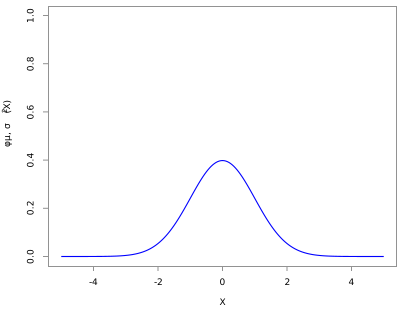
This curve is described by the so-called Gaussian function, which has the form:

$$f(x)=\frac{1}{\sigma \sqrt{2\pi }}{\mathrm{e}}^{-\frac{{(x-\mu )}^2}{2{\sigma }^2}}$$

The function is quite complicated, and you don't need to remember it. But we can see that the normal distribution is described by two parameters, the mean and the standard deviation (or variance). Different values of the mean and the standard deviation give different graphs:

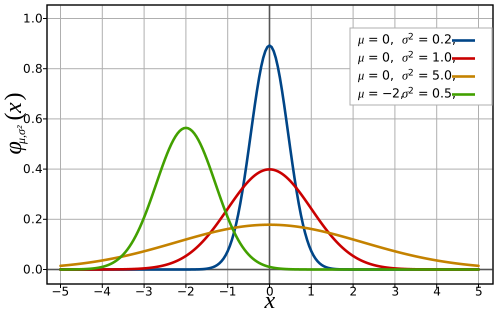
The normal distribution is important because it models quite faithfully many distributions that we can meet in real life. We can see that the curve always has a single global maximum, exactly at the mean. For example, the red curve has its maximum at X = 0, so the mean value of this quantity is zero. The curve is symmetrical: it has line symmetry about the line that is perpendicular to the X-axis and passes through the mean, that is, through the point X = 0. In other words, the curve looks the same to the left of zero as to the right of zero. The green curve has the same properties, but centred not on zero but on the point X = −2.

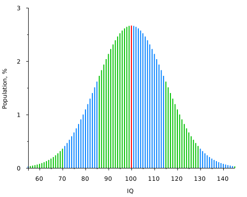
The normal distribution can describe the distribution of intelligence, or IQ, among people quite faithfully. By definition, the mean IQ is 100. About as many people have an IQ above 100 as below it. There are about as many people who are slightly below average as slightly above average, and as many dimwits as geniuses. Although it doesn't always look that way :-). A graph showing the approximate distribution of IQ:

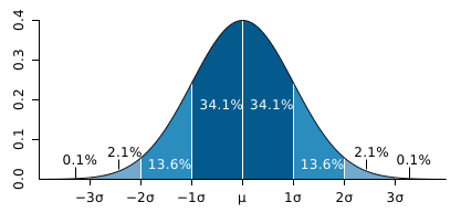
The standard deviation plays a big role in the normal distribution. If a distribution is normal and has standard deviation σ, then approximately 68% of the values lie in the interval [μ − σ, μ + σ]. In other words, roughly 68% of the values differ from the mean by at most one standard deviation. Approximately 95% of the values lie in the interval [μ − 2σ, μ + 2σ] and 99.7% of the values in the interval [μ − 3σ, μ + 3σ]. The following picture shows this clearly:

Links and sources

• Some of the images are from Wikipedia, from the articles Normal distribution and Intelligence.