Probability distribution

The probability distribution of a random variable tells us how likely it is that the random variable takes a particular value.

Distribution of a discrete variable

Let's take a discrete random variable. For example, we could record how many pints of beer the local drunk, Bertie, drinks in a day. By watching Bertie for a whole month, we put together the following table:

We can see that Bertie held back a little at the start of the month, but then he was knocking back one pint after another. And the week from day 11 must have been wild. Let's call this discrete random variable X. Now we want to know the probability that on any given day of the month Bertie drinks exactly x pints of beer.

Before we work out the probability itself, we draw an ordinary bar chart of frequencies. We find all the numbers of pints that Bertie drank on any day and put them on the chart. For example, Bertie drank ten pints on nine days in total, so for the value ten we will have a bar of height nine:

We read the chart like this: Bertie drank six pints on three days of the month.

What is the probability that Bertie drank ten pints in a day? Formally, we write it like this: we write the probability function as P, and the question about ten pints is written as P(X = 10). This asks: what is the probability that the random variable X takes the value ten?

The probability will be equal to the relative frequency of that value. So let's also draw a chart of the relative frequencies:

Now we can say that P(X = 10) is equal to 0.3, that is, 30%.

Experimental and theoretical probability

Let's take an ordinary dice and roll it 600 times. From the point of view of classical theoretical probability, we have an equal chance of getting a 1, a 2, …, a 6. Each face of the dice has a probability of $\frac{1}{6}$. In theory, then, each face should come up exactly 100 times when we roll the dice 600 times.

Of course, that most likely won't happen. In our experiment we might get these results:

We can see that the relative frequency, and so the experimental probability, of rolling a 1 is 0.175, which is 17.5%. That is close to the probability $\frac{1}{6}$, which is 0.16666…, but it is not quite exact.

That doesn't mean that one or the other probability is wrong. Making a perfectly balanced dice is not an easy task at all, and it can also be hard to carry out the test itself, rolling the dice 600 times.

Theoretical probability works under ideal conditions, where we would roll the dice forever. The longer we rolled an ideally balanced dice, the closer the relative frequencies of the individual scores would get to the theoretical probability.

That is why we distinguish two kinds of probability: theoretical probability, which comes from idealised conditions, and experimental probability (also called empirical probability), which we work out from the relative frequencies in our data.

To work out the experimental probability, we need a large enough data set. For example, we watched our drunk Bertie for only one month, but it would be much better to watch him for at least a year.

Distribution of a continuous variable

For a continuous variable we don't work out the probability at a single point, but always over an interval. The probability will be equal to the area under the curve, so to work it out we will need an integral. Here is a graph of a continuous variable, which could, for example, show measurements of some error in cm:

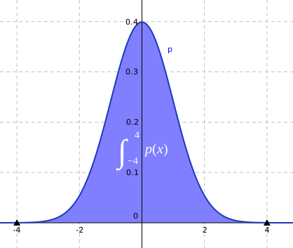
On the x-axis we have values in cm, and on the y-axis we have relative frequencies. Let's say we have measured only values in the interval [−4, 4]. The experimental probability that we measure an error in this interval is therefore 1, that is, 100%.

How does the area come into it? We say that the area ${\int }_{-4}^{4}p(x)$, where p is the probability function, gives us exactly that 100%. If we asked what the experimental probability is that the value lies in the interval [0, 4], we would get this picture:

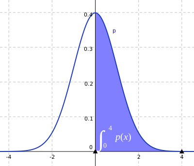
The previous shaded region corresponded to 100%, and this one corresponds to 50%, because its area is clearly half as big. To be precise, we would write the experimental probability as the ratio

$$\frac{{\int }_0^{4}p(x)}{{\int }_{-4}^{4}p(x)}.$$

The law of large numbers

The previous section is related to the well-known law of large numbers. Informally, it says that with a large number of independent trials, the relative frequency (experimental probability) gets closer to the theoretical probability.

We can picture this again with a coin toss. We can get heads or tails, and each side has a probability of $\frac{1}{2}$, or 50%. If we toss a coin four times, we might get heads three times and tails once. The relative frequencies are then $\frac{3}{4}$ and $\frac{1}{4}$. That is quite far from $\frac{1}{2}$.

If we toss it ten times in total, we might get heads seven times and tails three times. Those frequencies are $\frac{7}{10}$ and $\frac{3}{10}$. That is still a long way from $\frac{1}{2}$, but these numbers are closer to one half than the previous frequencies.

We could carry on like this. If we tossed a coin 1,000 times, we might get heads 520 times and tails 480 times. Those are the frequencies $\frac{13}{25}$ and $\frac{12}{25}$, which are already very close to one half (to give you an idea, $\frac{13}{25}=0.52$).

Notice that although the relative frequencies are much closer to one half, the frequencies themselves are much further from the “ideal” frequency. When we tossed the coin ten times, the ideal frequency for each side was 5. That is, we would get heads five times and tails five times. Since we got heads seven times, that gives a difference of two tosses: 7 − 5 = 2. We were “two tosses off” from what would happen in the ideal situation.

But when we tossed the coin 1,000 times, we got heads 520 times, which is a difference of 20 tosses from the ideal, because ideally each side should have come up 500 times. So it seems that the more times we toss, the further away our results get.

That doesn't matter at all: the law of large numbers does not claim that the frequencies will get closer to the ideal, only the relative frequencies. And those do get closer. So the frequencies may drift further away from the ideal, but the relative frequencies will get closer to it.