Linear functions
A linear function is any function given by the rule y = mx + b, where m and b are real numbers. A special case of a linear function occurs when m = 0, because then we can shorten the expression to y = b, which is a constant function (some sources don’t count a constant function as a linear function).
Types of linear functions
Linear functions have fairly nice graphs, because they are always described by a straight line. For example, the constant function mentioned above has a graph that is a line parallel to the x-axis, crossing the y-axis at b. If b = 0, the line always passes through the origin (0, 0). This function is also called direct proportion.
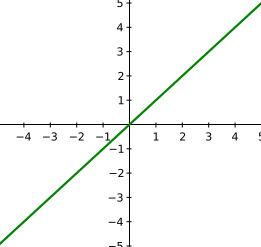
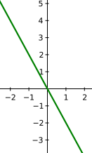
Other properties of a linear function follow from the value of m. If m > 0, the graph is that of an increasing function, but if m < 0, the graph is decreasing. The graph of y = mx is the reflection in the y-axis of the graph of y = −mx.
Properties of linear functions
If m ≠ 0, the domain of linear functions is the set of real numbers, and so is the range. The function is decreasing or increasing depending on the slope m. It is a one-to-one function, because we can’t find a horizontal line that crosses the graph of a linear function at more than one point. It is also not periodic, it is continuous on its whole domain, and it has no maximum or minimum. A linear function is neither even nor odd, except when b = 0, in which case it is an odd function.
Example
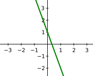
Draw the graph of the function y = −3x +1.
We can draw the graph of this function easily. We know that the graph of every linear function is a straight line (in theory it can also be a line segment, if you only have to draw the graph of a linear function on a particular interval). That’s all we need. To draw a straight line, we need to know the coordinates of just two points. Let’s work them out. First substitute the simplest number for x, zero. We get f(0) = 1. The first point the line passes through is (0, 1). For the second point we can substitute, say, one. We get this: f(1) = −3 + 1 = −2. The second point has coordinates (1, −2). Now we have the two points we need to draw the graph of this function: