Uniform motion in a straight line

On a motorway you switch on the cruise control at 108 km/h. The car is now going at the same speed all the time, straight ahead, and the needle of the speedometer does not move at all. How many metres does it cover in one second? Let’s convert the speed to metres per second, that is, divide by 3.6:

$$108\mathrm{km}/\mathrm{h}=\frac{108}{3.6}\mathrm{m}/\mathrm{s}=30\mathrm{m}/\mathrm{s}$$

Every second the car covers 30 m. In two seconds 60 m, in three 90 m, and so on and on, thirty metres more with every second.

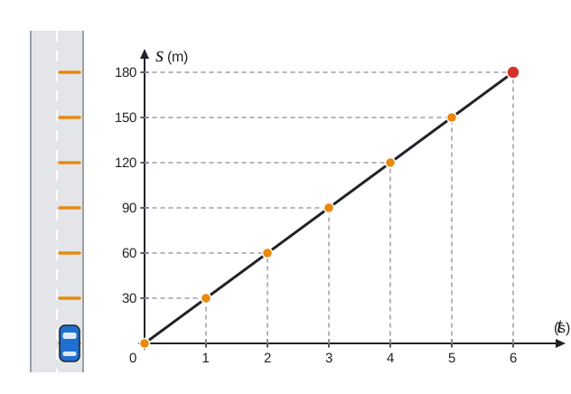
On the left we see the road from above, with the car driving up it. Every whole second our car leaves an orange mark on the road behind it, say a drop of paint. All the marks are the same distance apart, 30 m, because the car covers the same distance every second. On the right is the graph. On the horizontal axis is the time t in seconds, on the vertical axis the distance s in metres that the car has covered since the first mark. The vertical axis has the same scale as the road, so the red point in the graph always sits at the same height as the car. In the animation six seconds of driving pass, and with every second a mark is added on the road and an orange point in the graph.

Motion along a straight line in which the magnitude of the body’s velocity does not change is called uniform motion in a straight line. Motion in a straight line is motion whose path is a straight line. Uniform motion is motion in which the body covers equal distances in equal intervals of time, which is the same as a constant magnitude of the instantaneous speed. A car travelling at a constant speed along a straight line cannot turn, because it would leave the line, and it cannot turn back either, because it would have to slow down to zero to do so. So the direction of its velocity does not change either. Unlike the car on the roundabout, the whole velocity stays constant as a vector, that is, both its magnitude and its direction.

Nothing moves quite like this: there is always a little wind or the road rises uphill. But a car with cruise control on a straight motorway, an escalator on the Underground or a train on a straight track come very close to uniform motion in a straight line.

The formula for distance

If you are only looking for the formula, you calculate the distance s that a body covers in uniform motion at speed v in time t as

$$s=v\cdot t$$

We derive it from the formula for speed $v=\frac{s}{t}$, which we already know. All we need to do is multiply both sides by the time t:

$$\begin{array}{rcl}v& =& \frac{s}{t}/\cdot t\\ v\cdot t& =& s\end{array}$$

In plain words: if a car covers 30 m every second, in ten seconds it covers ten times as much. In a minute, that is in 60 s, the car with cruise control covers

$$s=30\mathrm{m}/\mathrm{s}\cdot 60\mathrm{s}=\mathrm{1,800}\mathrm{m}=1.8\mathrm{km}.$$

We calculate with units as we do with numbers. The seconds in the denominator cancel with the ones we multiply by, and metres are left:

$$\frac{\mathrm{m}}{\mathrm{s}}\cdot \mathrm{s}=\mathrm{m}$$

If you ended up with, say, metres times seconds, you would know that a mistake had been made somewhere.

Be careful, the formula s = v · t holds only for uniform motion. When the speed fluctuates, we do not know which of the speeds to put into the formula. Only the average speed helps us, $s=\overline{v}\cdot t$. The Smiths drove to Nottingham at an average of 82 km/h for 2.5 h, so they covered 82 km/h · 2.5 h = 205 km, even though their speedometer showed everything from zero to a hundred and thirty.

How long will it take?

When we divide the formula s = v · t by the speed v, we get the time:

$$t=\frac{s}{v}$$

The route from London to Nottingham along the M1 measures about 205 km. If the car travelled the whole way at a constant speed of 100 km/h, the journey would take

$$t=\frac{205\mathrm{km}}{100\mathrm{km}/\mathrm{h}}=2.05\mathrm{h}.$$

A motorway is not as straight as a ruler, but that does not bother the formula. Distance is measured along the path, so s = v · t holds for every uniform motion, even for a car that goes round bends at a constant speed.

How much is 2.05 h in hours and minutes? Certainly not two hours and five minutes. An hour has sixty minutes, not a hundred. We keep the two whole hours and convert the remaining five hundredths of an hour to minutes:

$$0.05\mathrm{h}=0.05\cdot 60\min =3\min$$

The journey would take 2 h and 3 min.

The third quantity remains, the speed. We calculate it with the formula $v=\frac{s}{t}$. Grace is cycling along a straight cycle path along the Thames at the same pace all the time and covers 6 km in 20 min. Twenty minutes is a third of an hour:

$$v=\frac{6\mathrm{km}}{\frac{1}{3}\mathrm{h}}=18\mathrm{km}/\mathrm{h}$$

Dividing by a third is the same as multiplying by three, which is why we got 6 · 3 = 18. If you do not like fractions, convert everything to metres and seconds. Twenty minutes is 20 · 60 s = 1,200 s:

$$v=\frac{\mathrm{6,000}\mathrm{m}}{\mathrm{1,200}\mathrm{s}}=5\mathrm{m}/\mathrm{s}$$

Both routes give the same result, because 5 m/s times 3.6 is 18 km/h.

The graph of distance is a straight line

Let’s write the distances of the car with cruise control from the introduction in a table:

Each row of the table is one point of the graph: we measure the time on the horizontal axis and the distance on the vertical one. This is exactly how the orange points in the animation above came about. They all lie on one straight line that starts at the origin. Why on a straight line?

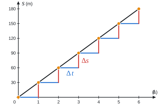
From each point to the next there is the same step: one second to the right (blue) and 30 m up (red). The steps are all equally wide and equally high, so the lines joining neighbouring points have the same slope (gradient) and join up without a kink. All the points therefore sit on one straight line. If the car had accelerated somewhere, there would be a higher step there and the line would bend upwards. The same holds between whole seconds. In half a second the car covers 15 m, in a tenth of a second 3 m, and all these points lie on the same straight line. That is why we draw the graph with a solid line, not just as seven dots.

We can tell how steep a line is from how much it rises when we move a little to the right. We write the width of a step, that is, the change in time, as Δt and the height of a step, the change in distance, as Δs. Their quotient gives the steepness:

$$\frac{\mathrm{\Delta }s}{\mathrm{\Delta }t}=\frac{30\mathrm{m}}{1\mathrm{s}}=30\mathrm{m}/\mathrm{s}$$

We got a number we already know: the speed of the car. The steepness of the distance–time graph is the speed. This is exactly the formula $v=\frac{\mathrm{\Delta }s}{\mathrm{\Delta }t}$ for instantaneous speed, only in uniform motion we do not have to take care that the section is short. If we take a bigger piece of the graph, the steepness comes out the same. Between the first and the fifth second 4 s passed and in them the car covered 150 m − 30 m = 120 m:

$$\frac{\mathrm{\Delta }s}{\mathrm{\Delta }t}=\frac{120\mathrm{m}}{4\mathrm{s}}=30\mathrm{m}/\mathrm{s}$$

A mathematician would say that distance is a linear function of time. Linear functions are written with the rule y = a · x + b and their graph is always a straight line. The number a says by how much y increases when x increases by one, and it is called the slope. The number b determines the height at which the line crosses the vertical axis, the y-intercept. Our formula s = v · t is a linear function in which time takes the place of x and distance the place of y, the slope is the speed and b = 0, so the line passes through the origin. Such a relationship is direct proportion: in twice the time the car covers twice the distance, in three times the time, three times the distance.

A faster car, a steeper graph

On a bridge our car with cruise control overtakes a lorry travelling at 72 km/h, that is

$$72\mathrm{km}/\mathrm{h}=\frac{72}{3.6}\mathrm{m}/\mathrm{s}=20\mathrm{m}/\mathrm{s}.$$

We will measure both time and distance from the bridge, and we will draw both graphs in one picture.

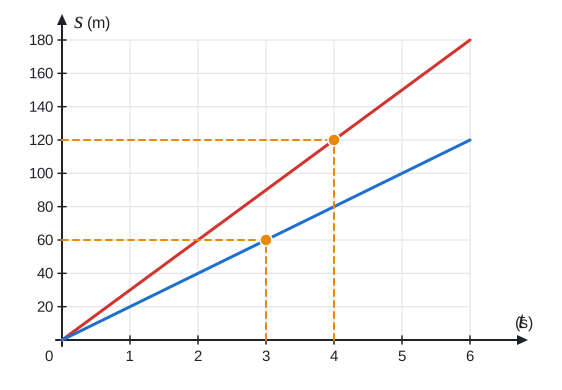
The red line of the car is steeper than the blue line of the lorry, because the car covers more every second. The steeper the distance–time graph, the faster the motion. If the lorry were standing still, its graph would be horizontal, with a steepness of zero.

We can also read values off the graph, which is why we have drawn a grid on it. Where will the lorry be after 3 s? We find three on the horizontal axis and climb up along the dashed line until we meet the blue line. From there we head left to the vertical axis and read 60 m. The other way round, we ask when the car will be 120 m beyond the bridge. We find 120 on the vertical axis, go right to the red line and then down to the time axis: after 4 s. We can check both with a calculation:

$$20\mathrm{m}/\mathrm{s}\cdot 3\mathrm{s}=60\mathrm{m},\frac{120\mathrm{m}}{30\mathrm{m}/\mathrm{s}}=4\mathrm{s}$$

The vertical distance between the lines shows how far the car is ahead of the lorry. After six seconds it is 180 m − 120 m = 60 m. The lead grows by 10 m every second, which is exactly the difference between the two speeds, 30 m/s − 20 m/s = 10 m/s.

When the car does not start from zero

So far we have measured distance from the place where we started the stopwatch. But we often start the stopwatch only when the body already has some of its journey behind it. Along the M1 there are marker posts, small signs with numbers that show how many kilometres it is from the start of the motorway in London. Near Watford a car passes the 21st kilometre and from that moment travels at a constant 90 km/h. At which kilometre will it be in two hours?

In two hours it covers 90 km/h · 2 h = 180 km. But the marker post will not show 180, because the car did not set off from zero. We calculate as if, at the moment we started the stopwatch, it already had 21 km behind it, because the marker post measures from the start of the motorway. This distance is called the initial distance and is denoted s₀. The distance at time t is then obtained by adding to the initial distance what the car has covered since the stopwatch was started:

$$s=s_0+v\cdot t$$

We substitute:

$$\begin{array}{rl}s& =21\mathrm{km}+90\mathrm{km}/\mathrm{h}\cdot 2\mathrm{h}\\ & =21\mathrm{km}+180\mathrm{km}=201\mathrm{km}\end{array}$$

In two hours the car will be at the 201st kilometre. When the initial distance is zero, we get the original formula s = v · t.

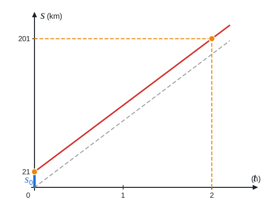
The graph no longer starts at the origin, but on the vertical axis at the height s₀ = 21 km, which the blue line segment shows. The steepness is still the speed, in every hour the graph rises by 90 km. The grey dashed line is the graph of a car that travels as fast but set off from the start of the motorway. The two lines are parallel, because they have the same steepness. The red one is just s₀ higher. In the language of the linear function y = a · x + b, a is the speed and b the initial distance.

Let’s turn it round: when will the car reach the 156th kilometre? It is tempting to divide 156 by ninety, but that would tell us how long it would take to get there from the start of the motorway. Instead we start from the formula and express the time from it:

$$\begin{array}{rcl}{s}_0+v\cdot t& =& s/-s_0\\ v\cdot t& =& s-s_0/:v\\ t& =& \frac{s-s_0}{v}\end{array}$$

We substitute:

$$t=\frac{156\mathrm{km}-21\mathrm{km}}{90\mathrm{km}/\mathrm{h}}=\frac{135\mathrm{km}}{90\mathrm{km}/\mathrm{h}}=1.5\mathrm{h}$$

The car reaches the 156th kilometre in an hour and a half, that is, in 1 h and 30 min.

Strictly speaking, the number on the marker post does not say what distance the car has covered, but where on the motorway it is. As long as the car only goes forwards, it is the same as the distance it would have covered from the start of the motorway. Why that matters we will see at the end of the article.

The speed–time graph

We can also draw speed in a graph. The car with cruise control goes at 30 m/s all the time, whatever the time, and so the graph of its speed is a horizontal line at height 30.

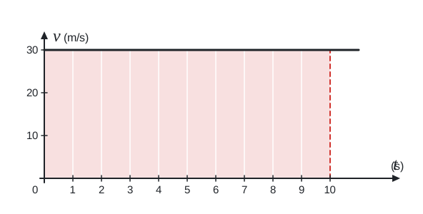
We will not find the distance on any axis of this graph. It is hidden in the area under the graph. Under the line, over the first ten seconds, there is a red rectangle 10 s wide and 30 m/s high. Its area, width times height, is

$$30\mathrm{m}/\mathrm{s}\cdot 10\mathrm{s}=300\mathrm{m}.$$

That is exactly the distance s = v · t that the car covers in ten seconds. Here the area does not come out in square metres but in metres, because the sides of the rectangle are not lengths but speed and time. The white lines divide the rectangle into ten strips, one for each second. Each has an area of 30 m/s · 1 s = 30 m, just as there are thirty metres between neighbouring marks on the road in the animation at the beginning.

Why bother with area when it is enough to multiply? Because the area under a speed–time graph means distance even when the graph is not horizontal. When we get to accelerated motion, the speed–time graph will rise and under it there will be a triangle or a trapezium instead of a rectangle. We will then calculate the distance as their area, and the formulae for the area of a triangle and a rectangle are enough, since a trapezium can be divided into them.

Standing still or going back?

In the morning Oscar sets off on his bike from home along a straight road. He rides for two hours at a constant speed of 20 km/h, then has lunch in a pub for an hour and finally rides home at the same speed.

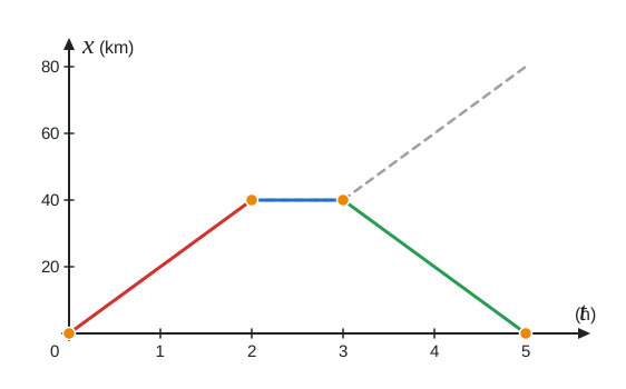
On the vertical axis this time there is not distance but position. We extend an x-axis along the road and put the origin at Oscar’s home. The position x then says how far along the road Oscar is from home, just as a marker post shows where on the road a car is. The grey dashed line is the distance that Oscar has ridden, which the cycle computer on the handlebars shows. Until the end of lunch it coincides with the position. We already know the red section. In two hours Oscar covers 40 km and the graph rises with a steepness of 20 km/h.

The blue section is horizontal. Time passes, but Oscar stays 40 km from home, so he is standing still. A horizontal graph means rest, the steepness is zero and so is the speed.

The green section goes down. Oscar is coming back and his position x decreases by 20 km every hour. A falling graph means motion backwards. We tell how fast Oscar is going from how much the graph falls in an hour, here by 20 km, so he rides at 20 km/h. His velocity now has the opposite direction from the morning. That is why physicists sometimes assign it a minus sign, which says that the position x decreases with time.

Now we can see why at the marker post we distinguished between where a body is and what distance it has covered. The cycle computer measures distance, and that never decreases with time. The dashed line therefore keeps rising after lunch and ends up at 80 km in the evening, whereas the graph of position ended at zero, because Oscar is home again. When travelling in one direction, position and distance differ only by the initial value, which is why the formula for distance s = s₀ + v · t was enough for the marker post. When a body turns round, we have to work with position.

Oscar’s whole trip is not uniform, it consists of three uniform pieces. The average speed for the whole day is the total distance divided by the total time, lunch included. The total distance is not the final position, which is zero. It is the 80 km where the dashed graph ends, that is 40 km + 0 km + 40 km:

$$\overline{v}=\frac{80\mathrm{km}}{5\mathrm{h}}=16\mathrm{km}/\mathrm{h}$$

There will never be a vertical section in the graph. It would mean that Oscar had moved some distance in zero time. And a graph that bent to the left would mean that time was running backwards for Oscar. So far nobody has managed either.

Calculator

The first calculator works out the distance from the speed and time, the second the time from the distance and speed. The pre-filled values come from the examples in the article: ten seconds with cruise control at 108 km/h and the journey from London to Nottingham at a steady hundred.

The formula s = s₀ + v · t and the distance–time graph can also be used to solve word problems in which one car catches up with another or two trains travel towards each other. Each vehicle has its own line in the graph and the place where they meet is the intersection of the lines. We will come to such problems later.

Before we start on them, the article How to solve kinematics and dynamics problems goes through a procedure that pays off with every physics problem: writing out the given information, converting units, a sketch and a general solution.